
Documentation
This guide covers the core MATLAB interfaces. For installation and a first estimate, see Getting started. The example manual (PDF) contains runnable examples, figures, and exercises.
Contents
- Dimension conventions
- State containers
- Dynamic models
- Observation models
- Least-squares estimation
- Recursive filtering
- Moment transforms
- Analysis and plotting
- API quick reference
- Example manual (PDF)
Dimension conventions
States, observations, and collections are columns. MATLAB uses one-based indices.
| Quantity | Shape |
|---|---|
| One state | n-by-1 |
| One observation | m-by-1 |
| State or sample collection | n-by-N |
| Predicted observations | m-by-N |
| Measurement Jacobian | m-by-n |
| Measurement covariance | m-by-m |
Estimators, likelihood evaluation, and filter measurement updates require a
single observation column. Trajectory means have shape n-by-N and their
covariances have shape n-by-n-by-N.
State containers
state = sftools.GaussianState([1; 2], diag([.5, .2]));
state.mean()
state.cov()

stream = RandStream('mt19937ar', 'Seed', 0);
particles = state.mean() + chol(state.cov(), 'lower')*randn(stream, 2, 500);
particleState = sftools.ParticleState(particles, -log(500)*ones(1, 500));

trajectory = sftools.StateTrajectory.preallocate(2, 5, true);
for k = 1:5
  trajectory.writeState(k, sftools.GaussianState(state.mean() + k - 1, state.cov()));
end
Output:
ans =

     1
     2


ans =

    0.5000         0
         0    0.2000
ParticleState stores particle columns and normalized log weights in
logWeights; its mean() and cov() return weighted empirical moments.
StateTrajectory is a handle object: writeState and writeMean modify it. Use
component(1) for the first component across time, stateAt(k) for one
sample, or preallocateLike to preserve an existing trajectory’s time grid.
iterSamples returns a cell array; sampleIterator offers lazy traversal
using hasNext() and next(). Either can include available covariance and
time metadata. For an available empty time vector, use zeros(1, 0);
[] denotes absent time metadata.
Dynamic models
Create models with sftools.createDynamicModel(name, ...). Arguments are
positional. Each provides f(x) for deterministic propagation, F(x) for its
Jacobian, G(x) for noise gain, and random(n, x, stream) for sampling.
| Name | State layout | Constructor arguments |
|---|---|---|
linear |
User-defined | F, G, Q |
cv |
Positions followed by velocities | T, Q, n |
ct |
[x; y; speed; heading; turn_rate] |
T, Q, n |
dyn = sftools.createDynamicModel('cv', .1, .01*eye(2), 2);
x = [0; 0; 1; .5];
predicted = dyn.f(x);
jacobian = dyn.F(x);
stream = RandStream('mt19937ar', 'Seed', 1);
samples = dyn.random(3, x, stream);
T is the sampling interval and Q the process-noise covariance.
The added state covariance is G(x)*Q*G(x).'.
Observation models
Create a model with sftools.createObservationModel(name, ...). Models
provide h(x), H(x), random(x, n, stream), and covariance R.
| Name | Measurement | Constructor arguments |
|---|---|---|
linear |
Linear mapping | H, R |
nonlinear |
User-provided mapping and Jacobian | h, H, R, ... |
pos |
Direct position observation | R, n |
toa |
Range to each anchor | p, R, n |
tdoa |
Range differences relative to first anchor | p, R, n |
tdoa_r0 |
Ranges with shared unknown offset | p, R, n |
anchors = [0, 10, 10, 0; 0, 0, 10, 10];
obs = sftools.createObservationModel('toa', anchors, .01*eye(4), 4);
x = [3; 4];
expected = obs.h(x);
jacobian = obs.H(x);
measurement = obs.random(x, 1, RandStream('mt19937ar', 'Seed', 2));
Anchors are columns of p. With n anchors, toa has n outputs and
tdoa has n-1. tdoa_r0 uses [x; y; r0] as its first state
components; additional state components have zero Jacobian columns.
Custom nonlinear h callbacks accept state batches and return measurement
columns, while H evaluates one state. Range Jacobians are undefined at
anchor positions, so choose linearization and initial points away from anchors.
Least-squares estimation
sftools.estimators.ls, wls, and nls return a GaussianState.
ls is unweighted and reports covariance using R; wls weights
residuals using the inverse of the measurement covariance R.
Both require a full-column-rank design matrix and pass
optional x0 only to model.H(x0). Use nls for nonlinear models.
For range localization, first run the example in
Observation models, then run:
initial = [5; 5];
estimate = sftools.estimators.nls(obs, measurement, initial);
disp(estimate.mean())
disp(estimate.cov())

fig = figure;
ax = axes(fig); hold(ax, 'on');
plot(ax, x(1), x(2), 'o', 'DisplayName', 'True position');
sftools.plotting.estimate(estimate, 'Axes', ax, ...
  'Confidence', .95, 'Label', 'NLS estimate');
xlabel(ax, 'Position x'); ylabel(ax, 'Position y');
axis(ax, 'equal'); legend(ax, 'show', 'Location', 'northoutside');
Output:
    3.1019
    3.9278

    0.0053   -0.0004
   -0.0004    0.0048
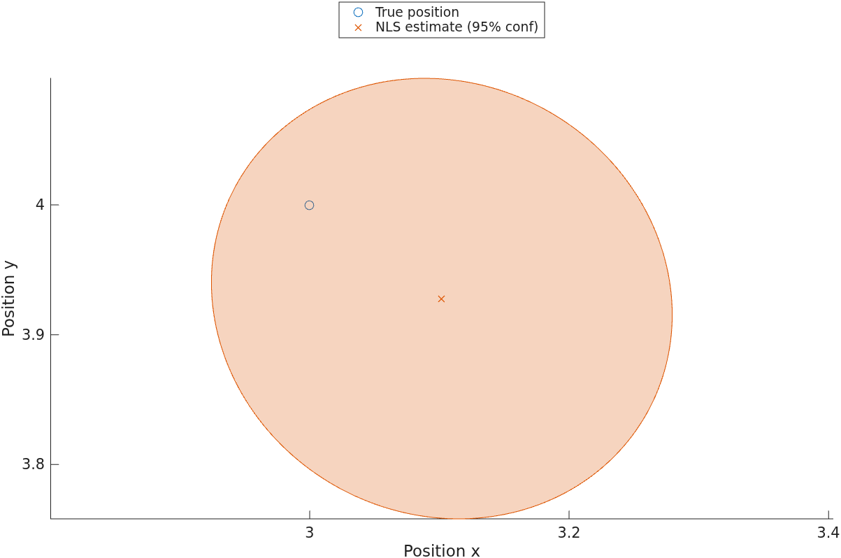
The plot zooms in on the estimated position; the four anchors are outside the displayed area. The ellipse shows the estimate’s local covariance.
nls uses analytic Jacobians and Optimization Toolbox when available, with
a base-MATLAB fallback otherwise. With one output, nonconvergence and
singular local covariance raise errors. With two outputs, either condition
returns an empty estimate and preserves optimizer diagnostics. A successful
fit and local covariance do not guarantee global optimality.
To retain optimizer diagnostics:
[fit, optimizer] = sftools.estimators.nls(obs, measurement, initial);
disp(optimizer.message)
if ~isempty(fit)
  disp(fit.mean())
  disp(fit.cov())
end
Output (the termination message depends on the available solver):
First-order optimality tolerance reached.
    3.1019
    3.9278

    0.0053   -0.0004
   -0.0004    0.0048
Recursive filtering
KalmanFilter requires linear dynamic and observation models.
ExtendedKalmanFilter handles nonlinear models; UnscentedKalmanFilter
uses sigma points, and ParticleFilter implements a bootstrap filter.
Each exposes measurementUpdate(state, obs, y) and timeUpdate(state).
There is deliberately no single call that runs the whole recursion:
you write the measurement and time updates explicitly.
- Understanding the two-stroke filtering engine. Each iteration incorporates an observation, records the posterior, then predicts the next state. The structure is the same for all filters.
- Flexible outlier rejection. Inspect each observation or innovation
and skip
measurementUpdatefor outliers, or treat them differently, using ordinary MATLAB code.
The example below follows that update-record-predict order:
stream = RandStream('mt19937ar', 'Seed', 4);
steps = 40;
dyn = sftools.createDynamicModel('cv', .1, .05*eye(2), 2);
obs = sftools.createObservationModel('pos', .4*eye(2), 2);
filter = sftools.filters.KalmanFilter(dyn);
truth = sftools.StateTrajectory.preallocate(4, steps, false);
estimates = sftools.StateTrajectory.preallocate(4, steps, true);
x = [0; 0; 1; .3];
state = sftools.GaussianState(zeros(4, 1), 8*eye(4));
for k = 1:steps
  truth.writeMean(k, x);
  y = obs.random(x, 1, stream);
  state = filter.measurementUpdate(state, obs, y);
  estimates.writeState(k, state);
  state = filter.timeUpdate(state);
  x = dyn.random(1, x, stream);
end
rmse = sqrt(mean((estimates.mean(1:2, :) - truth.mean(1:2, :)).^2, 'all'));
fprintf('Position RMSE: %.3f\n', rmse);
The example prints:
Position RMSE: 0.312
For particle filtering, initialize using initStateGaussian(mean, cov, n),
then explicitly call resample in the loop. Use an explicit RandStream for
repeatability; MATLAB and NumPy do not generate identical random sequences.
Moment transforms
| Function | Method |
|---|---|
sftools.transforms.ut(state, fun, ...) |
Unscented transform |
sftools.transforms.tt(state, {fun, jacobian, ...}) |
Taylor transform |
sftools.transforms.mct(state, fun, n, stream) |
Monte Carlo transform |
polar = sftools.GaussianState([10; .2], diag([.5^2, .05^2]));
toCartesian = @(x) [x(1, :).*cos(x(2, :)); x(1, :).*sin(x(2, :))];
ut = sftools.transforms.ut(polar, toCartesian);
mc = sftools.transforms.mct(polar, toCartesian, 20000, ...
  RandStream('mt19937ar', 'Seed', 3));
For tt, pass {f, F} for first-order propagation or {f, F, H} for
second order. Hessians use (state, state, output) ordering.
sigmaPoints exposes separate mean and covariance weights; additional
outputs from ut and mct retain the points or samples used. Monte Carlo
callbacks return one output column per input sample and need at least two
samples. Moment summaries do not establish that the distribution is Gaussian.
Analysis and plotting
sftools.analysis.llh(model, y, bounds, nPoints) evaluates a likelihood
map, and crlb(model, bounds, nPoints) evaluates a scalarized Cramer-Rao
bound. Bounds are [xmin, xmax; ymin, ymax], with upper limits excluded.
Undefined or rank-deficient CRLB points become NaN and cause a warning.
| Plot function | Purpose |
|---|---|
sftools.plotting.estimate |
Estimate and confidence ellipse |
sftools.plotting.signal |
One component and confidence band |
sftools.plotting.trajectory |
Two-dimensional trajectory and ellipses |
After running the example in Recursive filtering, plot the true and estimated trajectories:
fig = figure('Position', [100, 100, 1000, 400]);
layout = tiledlayout(fig, 1, 2);
axPath = nexttile(layout); hold(axPath, 'on');
sftools.plotting.trajectory(truth, 'Axes', axPath, ...
  'Select', [1, 2], 'Confidence', 0, 'Marker', 'none', 'Label', 'True');
sftools.plotting.trajectory(estimates, 'Axes', axPath, ...
  'Select', [1, 2], 'Confidence', 0, 'Marker', 'none', 'Label', 'KF estimate');
xlabel(axPath, 'Position x'); ylabel(axPath, 'Position y');
axis(axPath, 'equal'); legend(axPath, 'show');

axSignal = nexttile(layout); hold(axSignal, 'on');
sftools.plotting.signal(truth, 'Axes', axSignal, ...
  'Select', 1, 'Confidence', 0, 'Label', 'True');
sftools.plotting.signal(estimates, 'Axes', axSignal, ...
  'Select', 1, 'Confidence', .95, 'Label', 'KF estimate');
xlabel(axSignal, 'Time step'); ylabel(axSignal, 'Position x');
legend(axSignal, 'show');
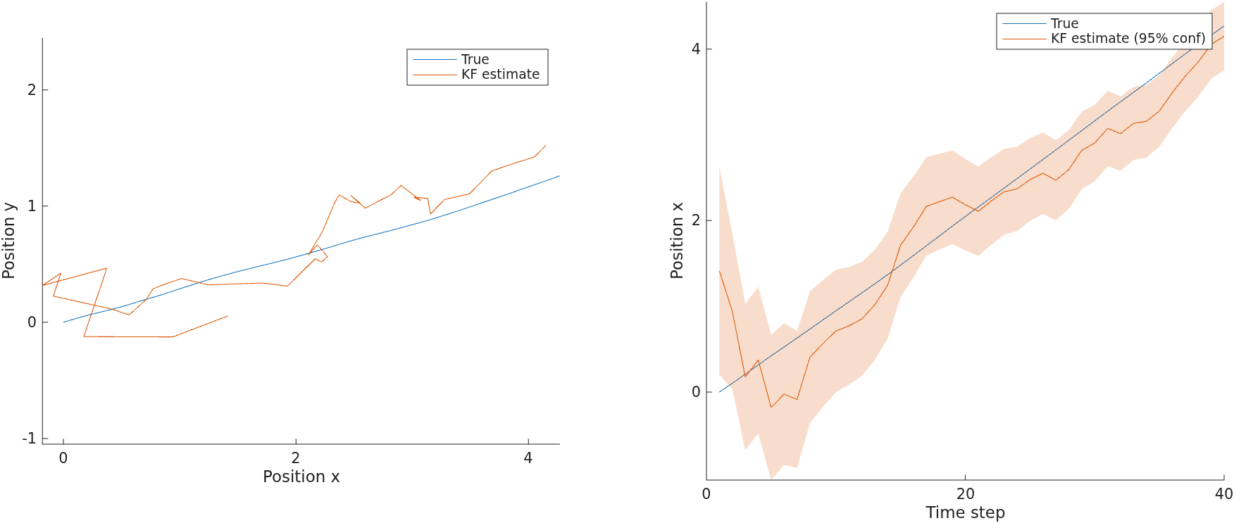
The left plot compares paths; the right shows the x position over time
and the filter’s 95% confidence band. For a state [x; y; vx; vy],
'Select', [1, 2] plots position and 'Select', [3, 4] plots velocity.
Options are MATLAB name-value pairs. Select uses one-based indices;
confidence visualization requires covariance data.
API quick reference
| Package | Interfaces |
|---|---|
sftools |
State containers, model factories, model registration |
sftools.models.dynamic |
Linear, CV, coordinated-turn |
sftools.models.observation |
Linear, nonlinear, position, TOA, TDOA, offset-range |
sftools.estimators |
ls, wls, nls |
sftools.filters |
Kalman, extended Kalman, unscented Kalman, particle |
sftools.transforms |
ut, tt, mct, sigmaPoints |
sftools.analysis |
llh, crlb |
sftools.plotting |
estimate, signal, trajectory |
For full signatures and failure modes, use MATLAB help, for example
help sftools.estimators.nls.
Example manual (PDF)
Download the example manual (PDF) for a more complete tutorial with worked examples, plots, and practice exercises on models, estimation, filtering, and moment transforms.